Chapter 6 Day 2 - Section 6 : Multivariate analysis and classification

6.1 Data

• The protein-level data quant.pd.rda from section 5.

---

6.2 Protein quantification

6.2.1 Read the protein level data from MSstatsTMT

library(tidyr)
library(dplyr)

# load data
load('data/data_ProteomeDiscoverer_TMT/quant.pd.rda')

# Pretend the two replicates within each condition and mixture are biological replicate
quant.pd <- quant.pd %>% 
  mutate(BioReplicate = paste(Mixture, Channel, sep="_"))

6.2.2 Protein quantification

We should first get subject quantification for each protein.

# protein quantification per subject
head(quant.pd)

# use technical replicate 2 and 3 as training data
quant.pd.per.subject <- quant.pd %>% filter(TechRepMixture != "1") %>% 
  group_by(Protein, BioReplicate) %>% 
  summarise(Abundance = median(Abundance, na.rm = TRUE)) %>%
  spread(BioReplicate, Abundance)

train_abun <- quant.pd.per.subject
colnames(train_abun)

# make protein abundance matrix
proteins <- train_abun$Protein
train_abun <- train_abun[, -1]
train_abun <- t(train_abun)
colnames(train_abun) <- proteins
dim(train_abun) # there are 50 rows (each row for subject) and 50 columns (one column per protein)

## [1] 50 50

# get annotation information
colnames(quant.pd)

## [1] "Run"            "Protein"        "Abundance"      "Channel"       
## [5] "BioReplicate"   "Condition"      "TechRepMixture" "Mixture"

train_anno <- quant.pd %>% select(BioReplicate, Condition)
train_anno <- unique(train_anno)
train_anno <- as.data.frame(train_anno)
dim(train_anno) # there are 50 rows (each row for subject)

## [1] 50  2

## remove the normalization channels
train_abun <- train_abun[train_anno$Condition != "Norm",]
train_anno <- train_anno[train_anno$Condition != "Norm",]

6.2.3 Deal with missing values

Please check whether there are missing values (NAs) or not. If there is no intensity at all in certain subject for certain protein, we can’t get subject-summarized for that run.

sum(is.na(train_abun))

## [1] 29

There are three NAs. Then, we need to decide how to deal with NAs. * First option: remove the samples with missing values * Second option: impute the missing values. Such as 1) with minimum value per protein or among all proteins, 2) with median or mean.

# First option: remove the samples with missing values
dim(na.omit(train_abun))

## [1] 22 50

# Second option: impute the missing values with miminal value
random.imp <- function (a){
  missing <- is.na(a)
  n.missing <- sum(missing)
  a.obs <- a[!missing]
  imputed <- a
  # imputed[missing] <- 0 # with zero
  # imputed[missing] <- median(a.obs) # with median values
  imputed[missing] <- min(a.obs) # with minimal values
  return (imputed)
}

pMiss <- function(x){
  sum(is.na(x))/length(x)*100
}

6.2.3.1 Only keep the subjects with less than 5% missing values

subjectmissing <- apply(train_abun, 1, pMiss)
train_abun <- train_abun[subjectmissing <= 5, ]
dim(train_abun)

## [1] 37 50

6.2.3.2 Impute the missing values

In this case, let’s impute the missing values with minimum value per protein.

# make sure the subject order in train_abun and train_anno consistent
train_anno <- train_anno[train_anno$BioReplicate %in% rownames(train_abun),] #remvoe the filtered subjects
train_abun <- train_abun[train_anno$BioReplicate,]

imputed_train_abun <- apply(train_abun, 2, function(x) random.imp(x))
imputed_train_abun <- as.data.frame(imputed_train_abun)

sum(is.na(imputed_train_abun))

## [1] 0

---

6.3 Principal components analysis (PCA)

6.3.1 PCA with prcomp function

Input has the row for run (subject) and the column for proteins.

?prcomp
# rows are proteins and columns are subjects
pc <- prcomp(imputed_train_abun)

# Inspect PCA object
summary(pc)

## Importance of components:
##                           PC1     PC2     PC3     PC4     PC5    PC6
## Standard deviation     2.6934 0.96718 0.52218 0.44114 0.41603 0.3419
## Proportion of Variance 0.7571 0.09762 0.02846 0.02031 0.01806 0.0122
## Cumulative Proportion  0.7571 0.85473 0.88318 0.90349 0.92155 0.9337
##                            PC7     PC8     PC9    PC10    PC11    PC12
## Standard deviation     0.31467 0.28257 0.26482 0.22441 0.22257 0.21286
## Proportion of Variance 0.01033 0.00833 0.00732 0.00526 0.00517 0.00473
## Cumulative Proportion  0.94408 0.95242 0.95974 0.96499 0.97016 0.97489
##                          PC13    PC14    PC15    PC16    PC17    PC18
## Standard deviation     0.1958 0.18588 0.16430 0.14277 0.13591 0.12553
## Proportion of Variance 0.0040 0.00361 0.00282 0.00213 0.00193 0.00164
## Cumulative Proportion  0.9789 0.98250 0.98532 0.98744 0.98937 0.99101
##                           PC19    PC20    PC21    PC22    PC23    PC24
## Standard deviation     0.12073 0.10874 0.10459 0.09577 0.08881 0.08152
## Proportion of Variance 0.00152 0.00123 0.00114 0.00096 0.00082 0.00069
## Cumulative Proportion  0.99254 0.99377 0.99491 0.99587 0.99669 0.99739
##                           PC25    PC26    PC27    PC28    PC29    PC30
## Standard deviation     0.07513 0.07431 0.06282 0.05512 0.05117 0.04461
## Proportion of Variance 0.00059 0.00058 0.00041 0.00032 0.00027 0.00021
## Cumulative Proportion  0.99797 0.99855 0.99896 0.99928 0.99955 0.99976
##                           PC31    PC32      PC33
## Standard deviation     0.04000 0.02629 2.325e-15
## Proportion of Variance 0.00017 0.00007 0.000e+00
## Cumulative Proportion  0.99993 1.00000 1.000e+00

names(pc)

## [1] "sdev"     "rotation" "center"   "scale"    "x"

6.3.2 Check the proportion of explained variance

Let’s check the proportion of explained variance. The first component has the largest variance. In this case, we need 2 components to capture most of the variation.

percent_var <- pc$sdev^2/sum(pc$sdev^2)
barplot(percent_var, xlab="Principle component", ylab="% of variance")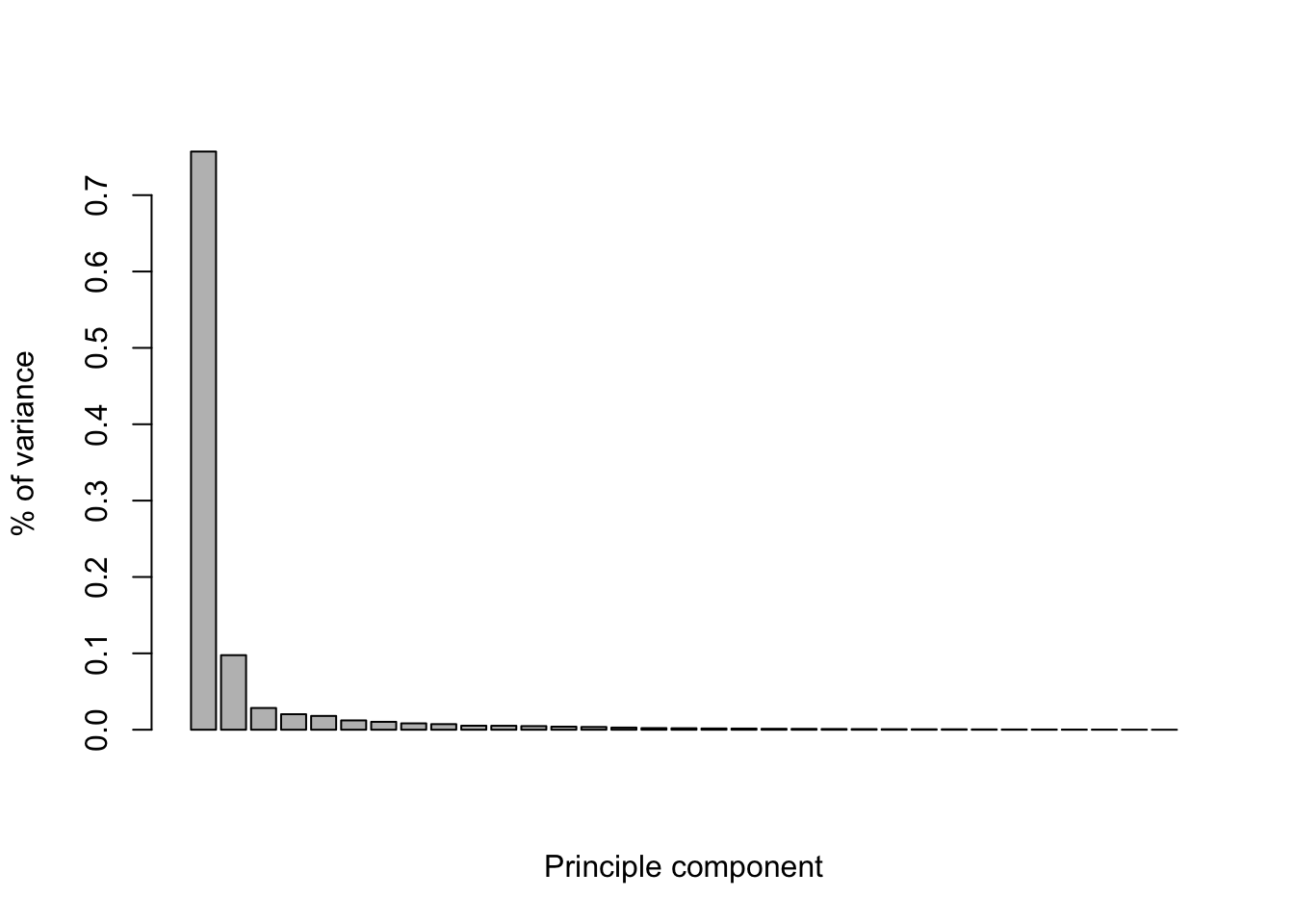

cum_var <- cumsum(pc$sdev^2/sum(pc$sdev^2))
barplot(cum_var, xlab="Principle component", ylab="Cumulative % of variance" )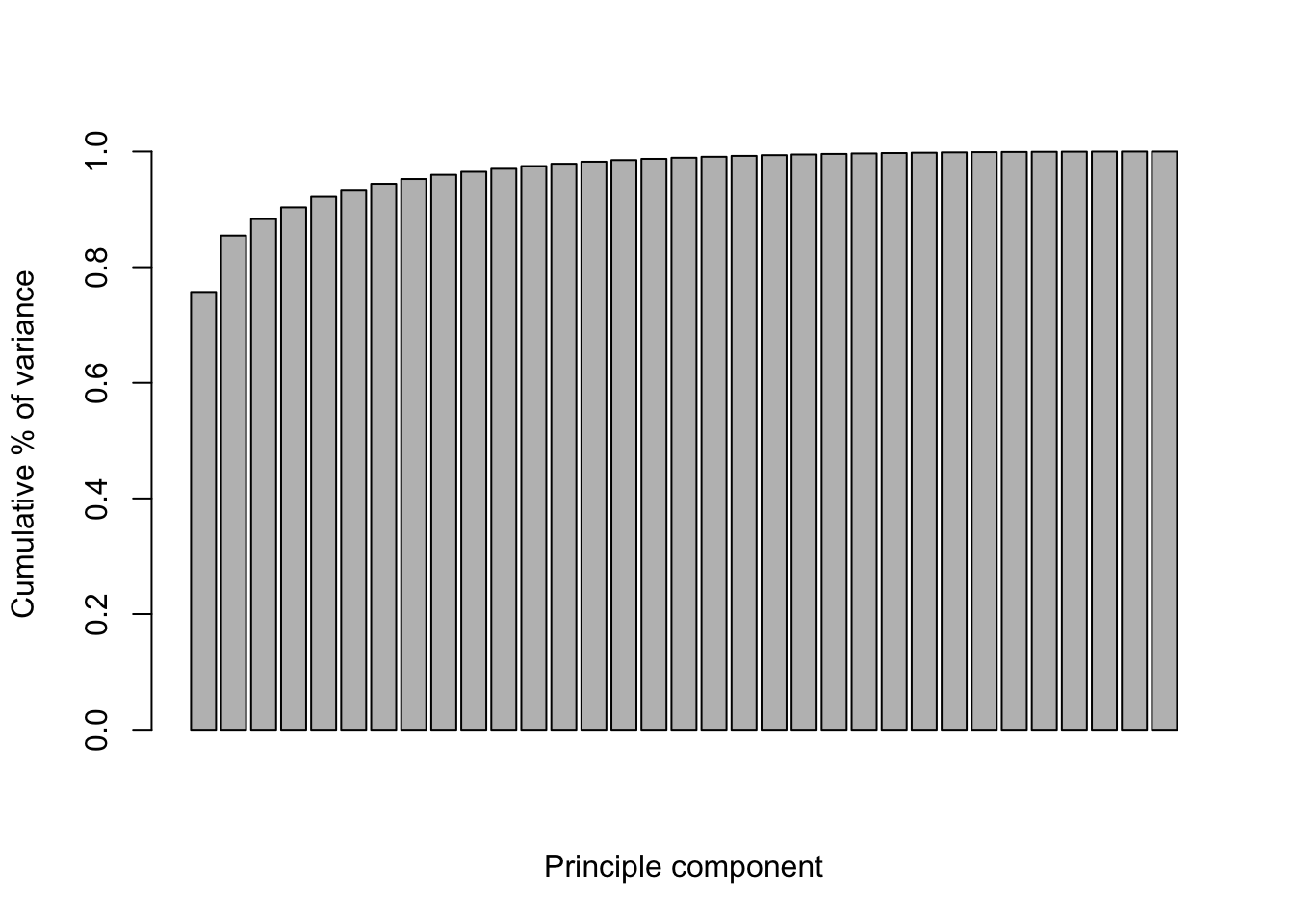

6.3.3 Visualization for PC1 vs PC2

Let’s visualize PC1 vs PC2 in scatterplot. ‘x’ include PC components for each subject.

# head(pc$x)
library(ggplot2)

ggplot(aes(x=PC1, y=PC2), data=data.frame(pc$x))+
  geom_point(size=4, alpha=0.5)+
  theme_bw()

In order to distinguish group by colors or shape, add Group informtion to ggplot. The order should be the same as column of input.

head(train_anno)

##    BioReplicate Condition
## 1 Mixture1_127C     0.125
## 2 Mixture1_129N     0.125
## 3 Mixture1_128N       0.5
## 4 Mixture1_129C       0.5
## 5 Mixture1_127N     0.667
## 6 Mixture1_130C     0.667

# Create PC1 vs PC2 scatterplot with Condition colors
ggplot(aes(x=PC1, y=PC2, color=Condition), data=data.frame(pc$x, Condition=train_anno$Condition))+
    geom_point(size=4, alpha=0.5)+
    theme_bw()

---

6.4 Heatmap

6.4.1 matrix format

ht.data <- t(imputed_train_abun)
# check the class
class(ht.data)

## [1] "matrix"

6.4.2 heatmap function in base stats package

First, let’s try to draw heatmap with base function.

# Change the font of row and column label
heatmap(ht.data, cexRow = 0.3, cexCol = 0.4)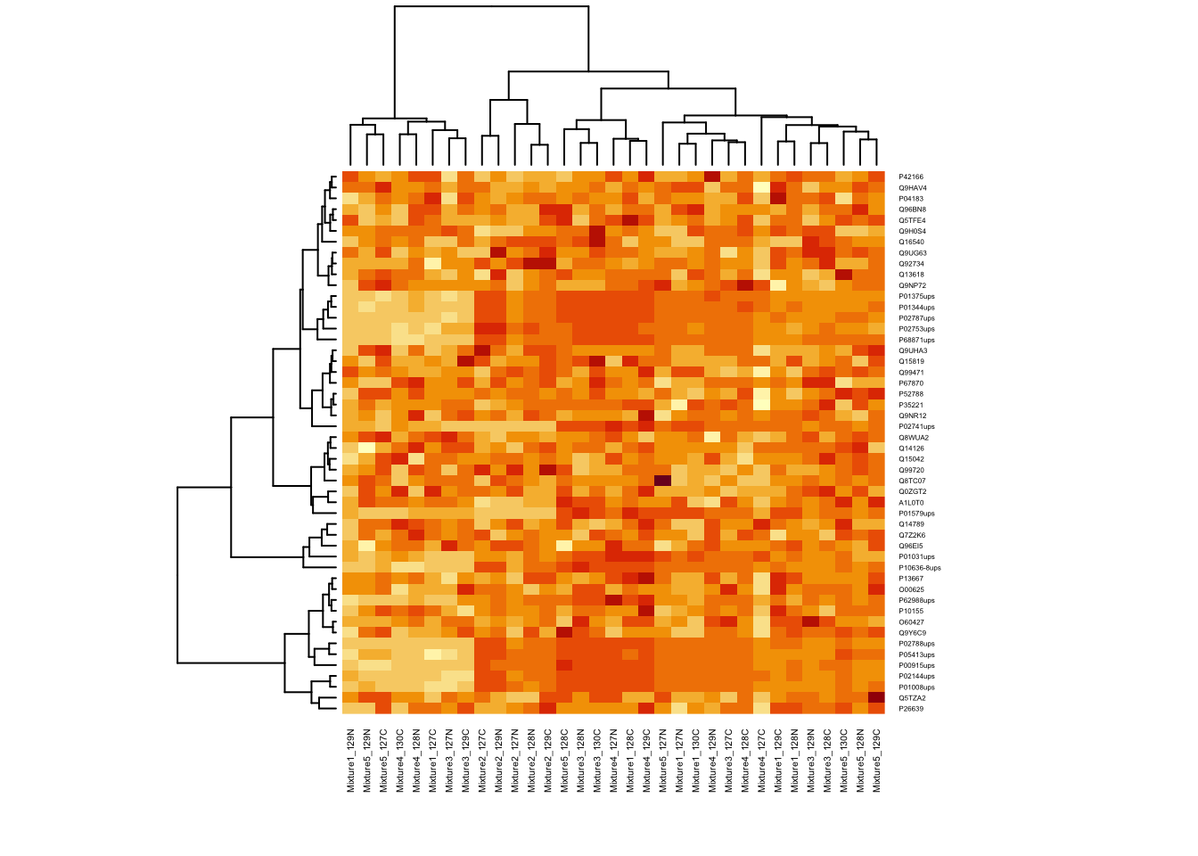

library(marray)

## Loading required package: limma

my.colors <- c(maPalette(low = "darkblue", high = "white", k = 7)[-7],
               "white", 
               maPalette(low = "white", high = "darkred", k = 7)[-1])

heatmap(ht.data, cexRow = 0.3, cexCol = 0.4, col = my.colors)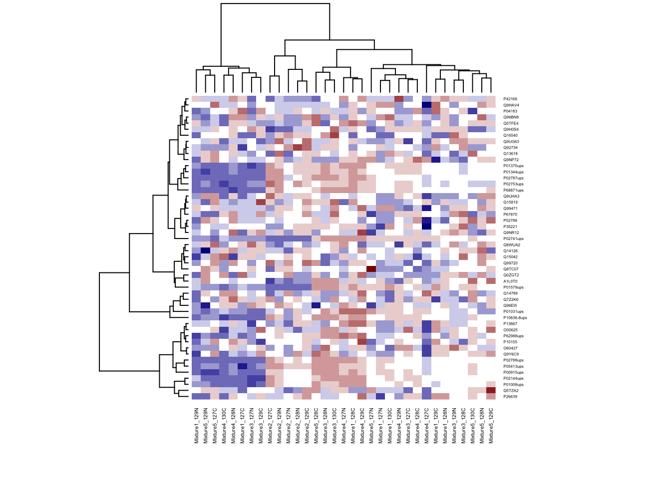

# Don't do cluster on rows
heatmap(ht.data, cexRow = 0.3, cexCol = 0.4, col = my.colors, Rowv = NA)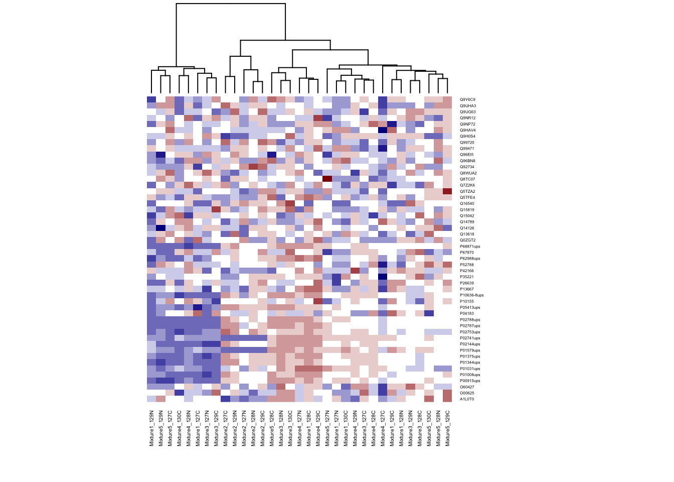

# Don't do cluster on columns
heatmap(ht.data, cexRow = 0.3, cexCol = 0.4, col = my.colors, Colv = NA)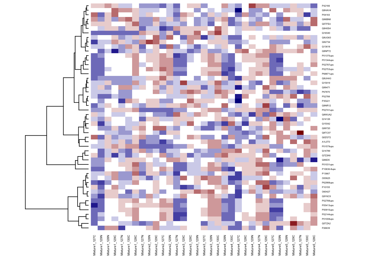

6.4.3 Color bar for group information

Add color side bar at th top of columns to distinguish group information by run.

unique(train_anno$Condition)

## [1] 0.125 0.5   0.667 1    
## Levels: 0.125 0.5 0.667 1 Norm

group.color <- rep("blue", nrow(imputed_train_abun))
group.color[train_anno$Condition == "1"] <- "red" 
group.color[train_anno$Condition == "0.667"] <- "yellow" 
group.color[train_anno$Condition == "0.5"] <- "orange" 
heatmap(ht.data, ColSideColors=group.color, col = my.colors, cexRow = 0.3, cexCol = 0.4, Rowv = NA)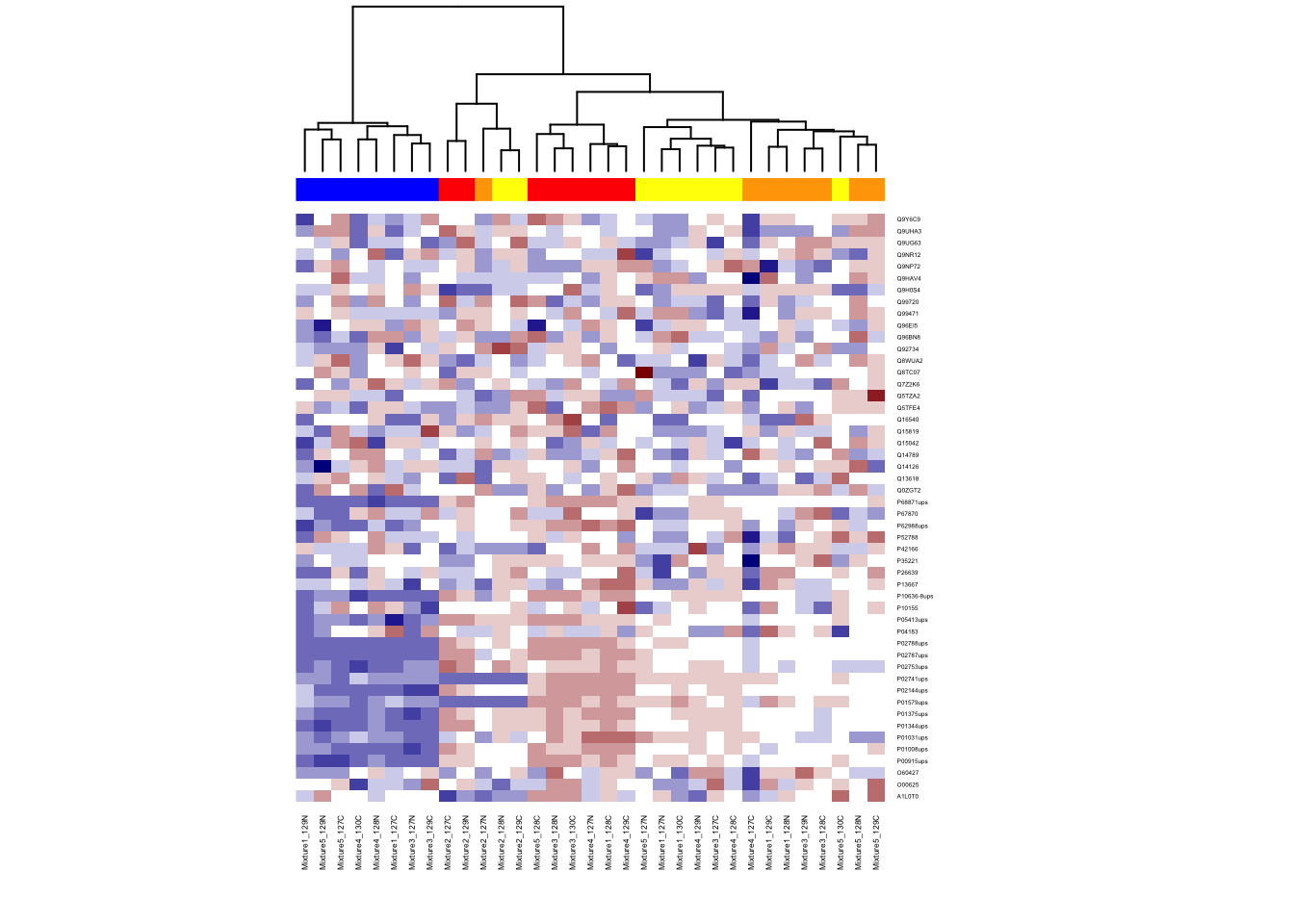

6.4.4 Different distance and clustering

Try different distances calculation and clustering methods. Choice of distance metric or clustering matters!

• Distance options: euclidean (default), maximum, canberra, binary, minkowski, manhattan

• Cluster options: complete (default), single, average, mcquitty, median, centroid, ward

# can change method for distance calculation
col_distance <- dist(t(ht.data), method = "euclidean")
# can change clustering method
col_cluster <- hclust(col_distance, method = "ward.D")

heatmap(ht.data,
        cexRow = 0.3, cexCol = 0.4, Rowv = NA, 
        ColSideColors = group.color,
        col = my.colors,
        Colv = as.dendrogram(col_cluster))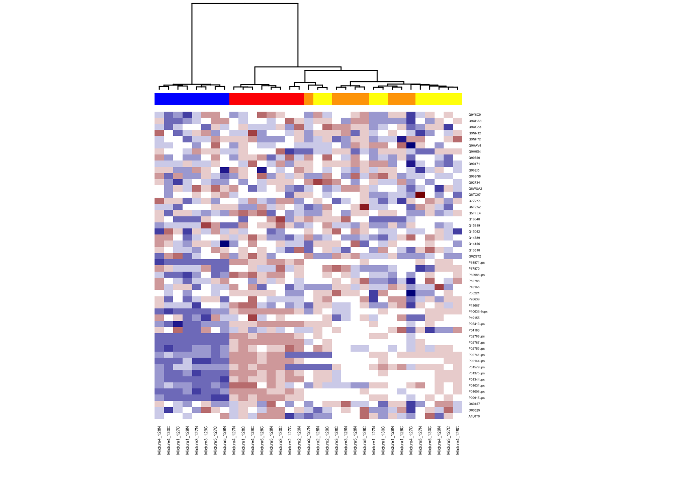 

---

6.5 Classification

6.5.1 Training random forest with all the proteins

Random Forest algorithm can be used for both classification and regression applications. In this tutorial, we will only focus random forest using R for binary classification example.

Random Forest algorithm is built in randomForest package of R and same name function allows us to use the Random Forest in R.

# Set random seed to make results reproducible:
set.seed(430)
#install.packages("randomForest")
# Load library
library(randomForest)
?randomForest

Some of the commonly used parameters of randomForest functions are

• formula : Random Forest Formula

• data: Input data frame

• ntree: Number of decision trees to be grown. Larger the tree, it will be more computationally expensive to build models.

• mtry: It refers to how many variables we should select at a node split. Also as mentioned above, the default value is p/3 for regression and sqrt(p) for classification. We should always try to avoid using smaller values of mtry to avoid overfitting.

• nodesize: nodesize - It refers to how many observations we want in the terminal nodes. This parameter is directly related to tree depth. Higher the number, lower the tree depth. With lower tree depth, the tree might even fail to recognize useful signals from the data. Defaut is 1 for classification.

• importance: Whether independent variable importance in random forest be assessed

Mainly, there are three parameters in the random forest algorithm which you should look at (for tuning): ntree, mtry and nodesize.

# add group information to the training data
imputed_train_abun$Condition <- droplevels(train_anno$Condition)

# randomForest dosen't allow special symbol in the protein name
colnames(imputed_train_abun) <- gsub("-", "", colnames(imputed_train_abun))

# fit random forest
rf=randomForest(Condition ~ . , data = imputed_train_abun, importance=TRUE)
rf

## 
## Call:
##  randomForest(formula = Condition ~ ., data = imputed_train_abun,      importance = TRUE) 
##                Type of random forest: classification
##                      Number of trees: 500
## No. of variables tried at each split: 7
## 
##         OOB estimate of  error rate: 0%
## Confusion matrix:
##       0.125 0.5 0.667 1 class.error
## 0.125     8   0     0 0           0
## 0.5       0   8     0 0           0
## 0.667     0   0     9 0           0
## 1         0   0     0 8           0

Variable importance plot is also a useful tool and can be plotted using varImpPlot function. Top 10 proteins are selected and plotted based on Model Accuracy and Gini value. We can also get a table with decreasing order of importance based on a measure (1 for model accuracy and 2 node impurity)

# plot importance of protiens
varImpPlot(rf, sort = T, 
           main="Variable Importance",
           n.var=10)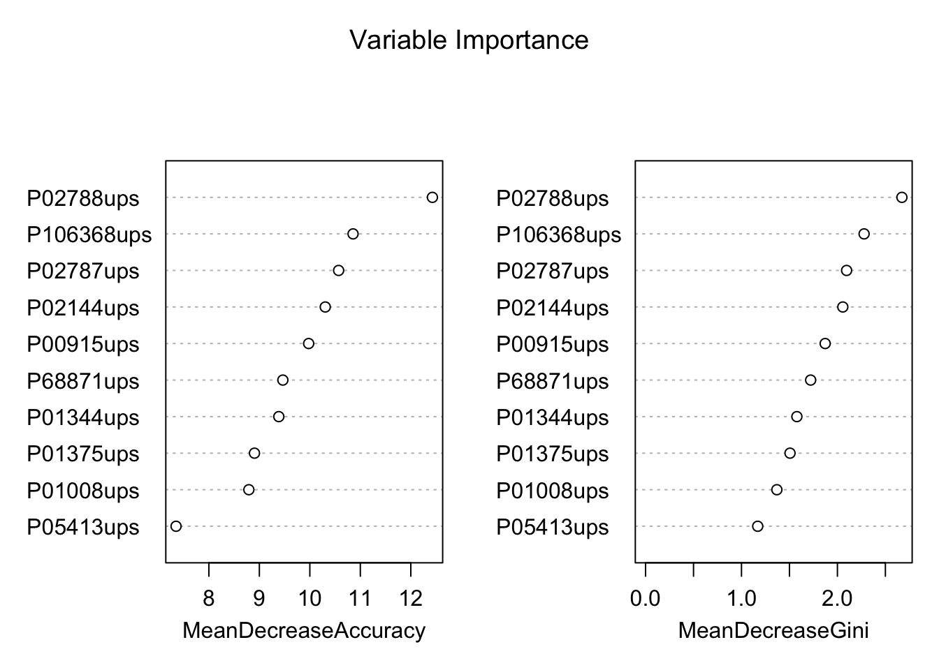

# store the importance of proteins 
var.imp <- data.frame(importance(rf,
                                 type=2))
# make row names as columns
var.imp$Variables <- row.names(var.imp)
# order the proteins based on their importance
var.imp <- var.imp[order(var.imp$MeanDecreaseGini,decreasing = T),]

# select top 10 proteins
biomarkers <- rownames(var.imp)[1:10]
biomarkers

##  [1] "P02788ups"  "P106368ups" "P02787ups"  "P02144ups"  "P00915ups" 
##  [6] "P68871ups"  "P01344ups"  "P01375ups"  "P01008ups"  "P05413ups"

6.5.2 Predict validation cohort

valid_abun <- quant.pd %>% filter(TechRepMixture == "1") %>% 
  select(Protein, BioReplicate, Abundance) %>%
  spread(BioReplicate, Abundance)

# make protein abundance matrix
proteins <- valid_abun$Protein
valid_abun <- valid_abun[, -1]
valid_abun <- t(valid_abun)
colnames(valid_abun) <- proteins
dim(valid_abun) # there are 50 rows (each row for subject) and 50 columns (one column per protein)

## [1] 50 50

# get annotation information
colnames(quant.pd)

## [1] "Run"            "Protein"        "Abundance"      "Channel"       
## [5] "BioReplicate"   "Condition"      "TechRepMixture" "Mixture"

valid_anno <- quant.pd %>% select(BioReplicate, Condition)
valid_anno <- unique(valid_anno)
valid_anno <- as.data.frame(valid_anno)
dim(valid_anno) # there are 50 rows (each row for subject)

## [1] 50  2

valid_abun <- valid_abun[valid_anno$BioReplicate,]
## remove the normalization channels
valid_abun <- valid_abun[valid_anno$Condition != "Norm",]
valid_anno <- valid_anno[valid_anno$Condition != "Norm",]

imputed_valid_abun <- apply(valid_abun, 2, function(x) random.imp(x))
imputed_valid_abun <- as.data.frame(imputed_valid_abun)
# randomForest dosen't allow special symbol in the protein name
colnames(imputed_valid_abun) <- gsub("-", "", colnames(imputed_valid_abun))

# prediction on validation set
valid_anno$Condition <- droplevels(valid_anno$Condition)
valid_pred <- predict(rf, imputed_valid_abun)

# Validation set assessment #1: looking at confusion matrix
table(data=valid_pred,
      reference=valid_anno$Condition)

##        reference
## data    0.125 0.5 0.667  1
##   0.125    10   0     0  0
##   0.5       0  10     2  0
##   0.667     0   0     8  0
##   1         0   0     0 10

# calculate the predictive accuracy
misClasificError <- mean(valid_pred != valid_anno$Condition)
print(paste('Accuracy',1-misClasificError))

## [1] "Accuracy 0.95"

The confusion matrix is a good way of looking at how good our classifier is performing when presented with new data.

---